Jane Street Puzzle - April 2025
puzzlesJane Street publish a puzzle every month or so. This is my solution for the April 2025 puzzle.
Problem
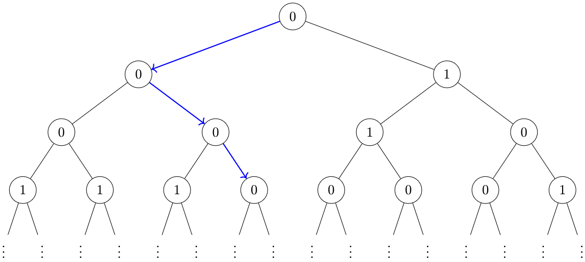
Figure 1: Example Binary Tree
For a fixed \(p\), independently label the nodes of an infinite complete binary tree \(0\) with probability \(p\), and \(1\) otherwise. For what \(p\) is there exactly a \(1/2\) probability that there exists an infinite path down the tree that sums to at most \(1\) (that is, all nodes visited, with the possible exception of one, will be labeled \(0\)). Find this value of \(p\) accurate to ten decimal places.
Approach
Since the problem is defined over an infinite binary tree, it feels natural to approach it recursively. Maybe we can set up a recurrence relation involving \(p\), and attempt to solve it? My first instinct was to try defining the probability of a “good” path (one with at most a single 1) in terms of the probabilities at the next level of the tree. After thinking it through more carefully, I realised that a recurrence based purely on tree layers wouldn’t capture the full picture. Since paths can share common prefixes, the recurrence needs to be defined at the level of individual nodes rather than entire layers. This way, we can correctly account for how the probability of a valid path depends on the structure and labels along shared parts of the tree.
Solution
Let \(n\) denote a node in a binary tree, with \(n.l\) / \(n.r\) representing the left left / right child nodes respectively. We denote a node’s label as \(n.x \; \in \; \{0, 1\} \).
Let’s reframe the problem. If there is at least one path where the sum is at most \(1\), this is the same as saying that not all the paths have a sum of at least 2.
We can formalise this idea. Define \(S(n)\) as the minimum path sum of a binary tree: \[S(n) \; = \; n.x \, + \, \min(S(n.l), \, S(n.r))\] In other words, \(S(n)\) represents the smallest possible sum along any infinite path that begins at node \(n\). This definition is naturally recursive: the minimum path sum at a given node is its value plus the smaller of the minimum path sums of its left and right children.
Suppose \(S(n) > 1\), this means the minimum path sum is strictly greater than \(1\), i.e. all paths have a sum of at least \(2\). We can now define the probability we aim to find. Given the root node \(n_{0}\), we are tasked with finding the probability \(1 - P(S(n_{0}) > 1)\).
Just like we defined \(S(n)\) recursively, we can define \(P(S(n) > 1)\) recursively: \[\begin{align*} P(S(n) > 1) =& \; p \, \cdot \, P(S(n.l) \, > 1) \, \cdot \, P(S(n.r) \, > 1) \, \cdot \\ & \; (1 - p) \cdot P(S(n.l) \, > 0) \cdot P(S(n.l) \, > 0) \end{align*}\]
Breaking this down, there’s a \(p\) chance that \(n.x = 0\). In this case, the current node contributes nothing to the minimum path sum, so both children’s minimum path sums must be strictly greater than \(1\), for \(n\)’s minimum path sum to be strictly greater than 1. Concretely, if \(n.x = 0\), then \(S(n) = \min(S(n.l), \, S(n.r)) > 1\) from which it follows that \(S(n.l) > 1\) and \(S(n.r) > 1\).
Similarly, there’s a \(1 - p\) chance that \(n.x = 1\). By applying similar reasoning, we can deduce that if this is the case, it must be that \(S(n.l) > 0\) and \(S(n.r) > 0\).
We can similarly derive a recursive definition for \(P(S(n) > 0)\): \[\begin{align*} P(S(n) > 0) =& \; p \, \cdot \, P(S(n.l) \, > 0) \, \cdot \, P(S(n.r) \, > 0) \, \cdot \\ & \; (1 - p) \end{align*}\]
We now note that since the trees are infinite, each subtree is similar to the parent tree. This gives us that \[\begin{align*} P(S(n) \, > 0) &= P(S(n.l) \, > 0) \\ &= P(S(n.r) \, > 0) \\ &= P \end{align*}\]
and
\[\begin{align*} P(S(n) \, > 1) &= P(S(n.l) \, > 1) \\ &= P(S(n.r) \, > 1) \\ &= Q \end{align*}\]
Note how we label these probabilities \(P\) and \(Q\) for clarity.
This allows us to rewrite / simplify our equations! We have that: \[\begin{align*} Q &= p \cdot Q^{2} \, + \, (1-p) \cdot P^{2} \\ P &= p \cdot P^{2} \, + \, (1-p) \end{align*}\]
We aim to find a value of \(p\) such that \(1 - P(S(n_{0}) > 1) = 1 - Q = 1/2\). This allows us to substitute \(Q = 1/2\) into our equations, yielding: \[\begin{align*} \frac{1}{2} &= \frac{p}{4} \, + \, (1-p) \cdot P^{2} \\ P &= p \cdot P^{2} \, + \, (1-p) \end{align*}\]
We have two equations with two unknowns. Solving this for a solution where \(p \in [0, 1]\) gives us the solution: \[p \approx 0.5306035754\]
Verifying the Solution with a Simulation
Before submitting my solution, I built a crude simulation of these randomly generated binary trees. Simulating trees of infinite depth is impossible, so as an approximation I chose to model trees of finite depth.
First I made a python class to randomly generate a tree of a given depth:
class BinaryTree:
    def __init__(self, p, depth):
        u = random.uniform(0, 1)
        if u <= p:
            self.x = 0
        else:
            self.x = 1
        if depth != 0:
            self.l = BinaryTree(p, depth - 1)
            self.r = BinaryTree(p, depth - 1)
        else:
            self.l = None
            self.r = None

    def min_path_sum(self):
        l = self.l.min_path_sum() if self.l is not None else 0
        r = self.r.min_path_sum() if self.r is not None else 0
        return self.x + min(l, r)
Then I repeatedly generated these binary trees, and measured the proportion of these trees which had a good path. I parallelised these experiments to speed up this process. Overall, it took around five minutes to run all of the iterations.
def run_single_simulation(p, depth):
    tree = BinaryTree(p, depth)
    return tree.min_path_sum() <= 1 # I.e. contains a "good" path


if __name__ == "__main__":

    # Converge to solution for p
    p = 0.5306035754

    # Verify solution by running simulation
    NUM_ITERATIONS = 1000
    TREE_DEPTH = 20

    with ProcessPoolExecutor() as executor:
        futures = [
            executor.submit(run_single_simulation, p, TREE_DEPTH)
            for _ in range(NUM_ITERATIONS)
        ]
        results = []
        for f in tqdm(futures):
            results.append(f.result())

    count = sum(results)
    print(count / NUM_ITERATIONS)
This gave me a number close enough to 0.5, which is what we were looking for!